- Load the R package we will use.
Question:
Modify the code for comparing differnet sample sizes from the virtual
bowlSegment 1: sample size = 26
1.a) Take 1100 samples of size of 26 instead of 1000 replicates of size 25 from the
bowldataset. Assign the output to virtual_samples_26virtual_samples_26 <- bowl %>% rep_sample_n(size = 26, reps = 1100)1.b) Compute resulting 1100 replicates of proportion red
-start with virtual_samples_26 THEN -group_by replicate THEN -create variable red equal to the sum of all the red balls -create variable prop_red equal to variable red / 26 -Assign the output to virtual_prop_red_26
virtual_prop_red_26 <- virtual_samples_26 %>%
  group_by(replicate) %>%
  summarize(red = sum(color == "red")) %>%
  mutate(prop_red = red / 26)
1.c) Plot distribution of virtual_prop_red_26 via a histogram
use labs to
-label x axis = “Proportion of 26 balls that were red” -create title = “26”
ggplot(virtual_prop_red_26, aes(x = prop_red)) +
  geom_histogram(binwidth = 0.05, boundary = 0.4, color = "white") +
  labs(x = "Proportion of 26 balls that were red", title = "26")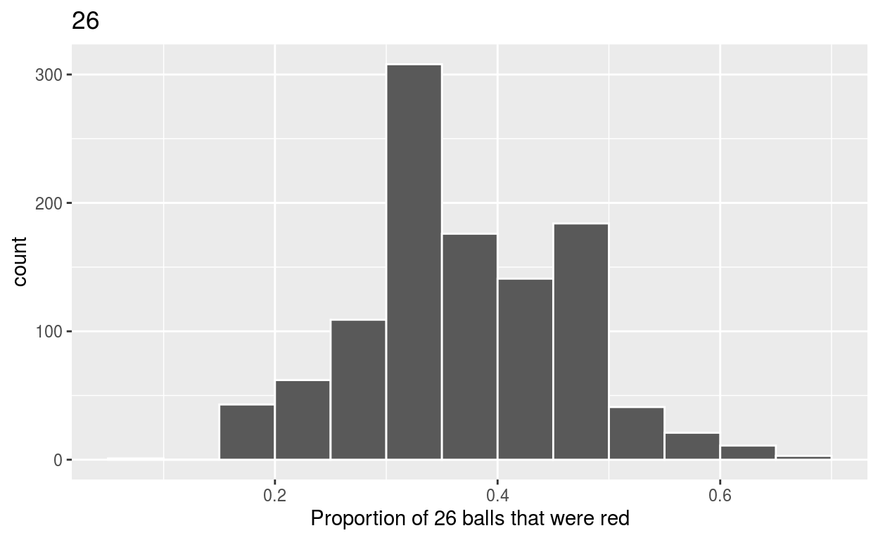
Segment 2: sample size = 57
2.a) Take 1100 samples of size of 57 instead of 1000 replicates of size 50. Assign the output to virtual_samples_57
virtual_samples_57 <- bowl %>%
  rep_sample_n(size = 57, reps = 1100)
2.b) Compute resulting 1100 replicates of proportion red
-start with virtual_samples_57 THEN -group_by replicate THEN -create variable red equal to the sum of all the red balls -create variable prop_red equal to variable red / 57 -Assign the output to virtual_prop_red_57
virtual_prop_red_57 <- virtual_samples_57 %>%
  group_by(replicate) %>%
  summarize(red = sum(color == "red")) %>%
  mutate(prop_red = red / 57)
2.c) Plot distribution of virtual_prop_red_57 via a histogram
use labs to
-label x axis = “Proportion of 57 balls that were red” -create title = “57”
ggplot(virtual_prop_red_57, aes(x = prop_red)) +
  geom_histogram(binwidth = 0.05, boundary = 0.4, color = "white") +
  labs(x = "Proportion of 57 balls that were red", title = "57")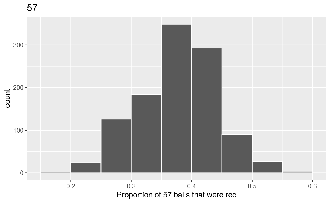
Segment 3: sample size = 110
3.a) Take 1100 samples of size of 110 instead of 1000 replicates of size 50. Assign the output to virtual_samples_110
virtual_samples_110 <- bowl %>%
  rep_sample_n(size = 110, reps = 1100)
3.b) Compute resulting 1100 replicates of proportion red
start with virtual_samples_110 group_by replicate THEN create variable red equal to the sum of all the red balls create variable prop_red equal to variable red / 110 Assign the output to virtual_prop_red_110
virtual_prop_red_110 <- virtual_samples_110 %>%
  group_by(replicate) %>%
  summarize(red = sum(color == "red")) %>%
  mutate(prop_red = red / 110)
3.c) Plot distribution of virtual_prop_red_110 via a histogram
use labs to
-label x axis = “Proportion of 110 balls that were red” -create title = “110”
ggplot(virtual_prop_red_110, aes(x = prop_red)) +
  geom_histogram(binwidth = 0.05, boundary = 0.4, color = "white") +
  labs(x = "Proportion of 110 balls that were red", title = "110")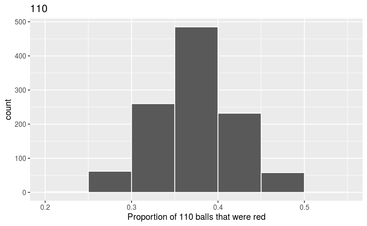
ggsave(filename = "preview.png",
       path = here::here("_posts", "2021-05-04-sampling"))
Calculate the standard deviations for your three sets of 1100 values of
prop_redusing thestandard deviationn = 26
virtual_prop_red_26 %>%
  summarize(sd = sd(prop_red))
# A tibble: 1 x 1 sd <dbl> 1 0.0959n = 57
virtual_prop_red_57 %>%
  summarize(sd = sd(prop_red))
# A tibble: 1 x 1 sd <dbl> 1 0.0632n = 110
virtual_prop_red_110 %>%
  summarize(sd = sd(prop_red))
# A tibble: 1 x 1 sd <dbl> 1 0.0458The distribution with sample size, n = 110, has the smallest standard deviation (spread) around the estimated proportion of red balls.